
If you’ve ever tried to analyse data from multiple tables in Excel using only VLOOKUP or INDEX-MATCH, you already know how quickly things can get messy.
Slow calculations, broken formulas, and file bloat become the norm once your dataset grows beyond a few thousand rows.
But Excel has evolved far beyond a simple spreadsheet tool. Today, it functions as a powerful data analysis platform, especially when you start using Power Pivot relationships.
In this guide, I’ll show you how Excel Power Pivot relationships let you connect multiple tables inside a single data model.
You’ll learn why this approach replaces traditional lookup formulas, how to build relationships step by step, and what mistakes to avoid.
What is Power Pivot in Excel?
Power Pivot in Excel is an advanced data modelling and analysis feature. It allows you to import millions of rows from multiple sources: databases, Excel tables, text files, or even cloud services, and then create relationships between those tables.
Unlike a normal worksheet, Power Pivot stores data in a compressed, column-based engine. This means you can analyse large datasets without slowing down your workbook or writing complex nested formulas.
Key benefits of Power Pivot:
- Handles up to millions of rows efficiently
- Compresses data to reduce file size
- Works with multiple data sources simultaneously
Think of Power Pivot as your gateway to building real relational data models inside Excel.
But before we dive into relationships, let’s first understand what a data model actually is, because Power Pivot is just the engine that powers it.
What Are Data Models in Excel?
A data model in Excel is a structured way of connecting multiple datasets together. Instead of flattening everything into a single giant table, you keep each logical set of data separate.
For example:
- One table for sales transactions
- One table for product details
- One table for customer information
These tables link through Excel data model relationships using common fields like ProductID or CustomerID.
Once linked, Excel understands how the tables relate to one another. You can then build PivotTables, write DAX formulas, and create dashboards that pull data from all connected tables simultaneously.
In short, a data model turns Excel into a relational database.
So why go through the trouble of building a data model? Because relationships between tables are what make this structure truly powerful. Let us explain why they matter.
Why Power Pivot Relationships Are Important?
Here’s the reality: most real-world data does not live in one perfect table.
- Sales data lives in one file
- Product details live in another
- Customer regions might live in a third
Without relationships, you’d copy, paste, and look up values across sheets—repetitive, error-prone, and slow.
Power Pivot relationships solve this by connecting datasets directly. When you link sales to products, Excel knows that every SaleID belongs to a specific ProductName. That means you can analyse revenue by product category without ever writing a VLOOKUP.
Why this matters:
- Eliminates repetitive lookup formulas
- Reduces errors from manual data merging
- Improves calculation speed across large datasets
Relationships let Excel do the heavy lifting so you focus on insights, not formula debugging.
Now that you understand why relationships are essential, let’s look at the different types you’ll encounter when building your data model.
Types of Relationships in Power Pivot
When you build a Power Pivot data model, you’ll encounter three main types of relationships.
1. One-to-Many (Most Common)
One record in a table links to many records in another table. For example, one customer (unique CustomerID) can have many sales transactions. This is your standard relationship between dimension tables (customers, products) and fact tables (sales).
2. Many-to-One
The same as above, but viewed from the opposite direction. Many sales point back to one product.
3. Many-to-Many
This occurs when multiple records in one table relate to multiple records in another. For example, products and salespeople where a salesperson sells many products, and each product is sold by many salespeople.
Pro Tip
While many-to-many is possible, it can cause ambiguous results unless handled carefully with DAX. In most Excel data models, stick to one-to-many relationships for clarity and performance.
Knowing the types is one thing, but how do you actually go about creating these relationships in Power Pivot? Let’s walk through the process step by step.
How to Create Relationships in Power Pivot
Creating relationships in Power Pivot is straightforward once you know the steps.
Here’s a practical, action‑oriented guide to get you from imported tables to a fully connected data model:
Step 1 – Import your tables
- Go to Power Pivot > Manage > Get External Data.
- Import all the tables you need; for example, Sales, Products, and Customers.
Step 2 – Identify unique keys
- Check that each table has a column with unique, non‑duplicate values.
- In Products, ProductID must be unique. In Sales, ProductID can repeat.
Step 3 – Create the relationship
- In Power Pivot, go to Diagram View (the icon on the top right).
- Drag from the key column in one table to the matching column in another.
- For example, drag Sales[ProductID] to Products[ProductID].
Step 4 – Verify the relationship
- Power Pivot draws a line between the tables.
- Click the line to see the direction (one-to-many).
- Confirm that the join works by creating a PivotTable using fields from both tables.
Quick checklist before creating relationships:
- Key columns have unique values on the “one” side
- Matching columns have the same data format (both text or both numbers)
- No blank values in key columns
Pro tip: Always ensure matching columns have the same data format. If one is text and the other is a number, Power Pivot won’t create the relationship.
Theory is helpful, but nothing beats a concrete example. Here’s an example of what a fully connected Power Pivot data model looks like in action.
Example of a Power Pivot Data Model
Here’s a simple Power Pivot data model in action:
Imagine you have three separate tables: Sales, Products, and Customers.
Sales Table

Product Table

Customers Table

Connect Them In Power Pivot
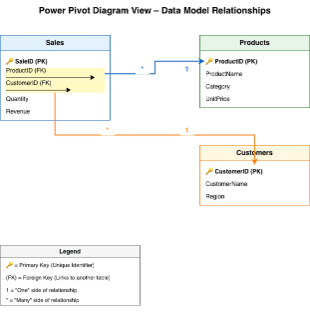
Two simple drag‑and‑drop steps:
- Drag from Sales[ProductID] → Products[ProductID]
- Drag from Sales[CustomerID] → Customers[CustomerID]
Power Pivot draws the lines. Your data model is ready.
The Result – A PivotTable Across All Three Tables
To build it:
- Insert > PivotTable → check “Use this workbook’s Data Model”
- Drag Category (from Products) to Rows
- Drag Region (from Customers) to Columns
- Drag Revenue (from Sales) to Values
Excel instantly returns:
| East | West | Grand Total | |
| Accessories | 300 | 300 | |
| Electronics | 500 | 750 | 1,250 |
| Grand Total | 800 | 750 | 1,550 |
That’s it. No VLOOKUPs. No broken formulas. Just three tables, two relationships, and one PivotTable that pulls everything together.
By now, you’re probably seeing the potential. But let’s make it crystal clear: what specific advantages do Power Pivot relationships give you over traditional Excel methods?
Advantages of Using Power Pivot Relationships
Why should you move from traditional formulas to Power Pivot for data analysis? Here are the key benefits.
1. Performance Benefits
- Handles millions of rows without freezing Excel
- Compressed data storage reduces file size
- In-memory calculations run much faster than worksheet formulas
2. Workflow Benefits
- No more dragging VLOOKUP formulas down 100,000 rows
- Build PivotTables that pull from multiple tables simultaneously
- Update one source table, and all reports refresh together
3. Reliability Benefits
- Eliminates #N/A errors from broken lookups
- Removes manual copying and pasting between sheets
- Creates a single source of truth for your analysis
If you’re building dashboards or recurring reports, Power Pivot relationships save you hours every week.
Of course, no tool is without its pitfalls. Even seasoned users make mistakes when setting up relationships, so let’s look at the most common ones and how you can avoid them.
Common Mistakes When Creating Power Pivot Relationships
Even experienced users make errors when building Excel Power Pivot relationships. Here are the most common mistakes and how to avoid them.
1. Duplicate Values In Key Columns
- What happens: Power Pivot cannot create a clean relationship. It may show an error or create a many-to-many relationship by accident.
- How to fix it: Always use unique identifier columns on the “one” side of the relationship (like ProductID in your Products table). Use Excel’s Remove Duplicates feature before importing.
2. Incorrect Relationship Direction
- What happens: Your PivotTable shows wrong totals or blank values. The relationship might be backwards (one-to-many instead of many-to-one).
- How to fix it: In Diagram View, the arrow should point from the many side (Sales) toward the one side (Products). Click the line to verify direction.
- Make sure the lookup table (such as Products) has unique values in the key column, and the transaction table (such as Sales) contains the repeating matching values.
3. Many-To-Many Relationships Without a Bridge Table
- What happens: Results become ambiguous. Excel doesn’t know which path to follow, so your PivotTable totals may double-count or show unexpected numbers.
- How to fix it: Avoid many-to-many in simple models. It is usually better to resolve many-to-many structures using a bridge table rather than relying on a direct many-to-many design.
4. Mismatched Data Formats Between Columns
- What happens: Power Pivot won’t let you create the relationship at all. The columns look identical, but one is text, and one is a number.
- How to fix it: Before importing, ensure matching columns have the same format. Use Excel’s Text to Columns or format cells consistently.
5. Blank Values in Key Columns
- What happens: The relationship works partially, but rows with blank keys get excluded from your PivotTable results without warning due to unmatched rows.
- How to fix it: Fill or remove blanks before importing. Use Find & Select > Go To Special > Blanks to locate them quickly.
6. Creating Relationships on Non-Key Columns
- What happens: The relationship is created successfully, but your PivotTable results don’t make sense – because the columns you linked aren’t true identifiers.
- How to fix it: Only link unique identifier columns (like ProductID or CustomerID). Never link columns like ProductName or CustomerName – names can repeat or change.
Quick Checklist – Before You Create a Relationship
- The “one” side column has unique values (no duplicates)
- Both columns have the same data format (text + text, or number + number)
- No blank values in either column
- You’re linking true identifier columns, not descriptive ones
- The arrow in Diagram View points many → one (Sales → Products)
Bottom line: Clean data leads to clean relationships. Most mistakes happen before you even open Power Pivot. Fix your source tables first, and Power Pivot will work flawlessly.
At this point, you might be wondering: if Power Pivot relationships are so powerful, do traditional Excel formulas still have a place? Let’s compare them head‑to‑head.
Power Pivot vs Traditional Excel Formulas
Let’s settle the debate: Power Pivot vs traditional Excel formulas.
| Aspect | Traditional Excel (VLOOKUP, XLOOKUP, INDEX-MATCH) | Power Pivot Relationships |
| Data size | Slows down beyond 50,000 rows | Handles millions of rows easily |
| Multiple tables | Requires merging or repeated lookups | Connects tables natively |
| Formula complexity | Long, nested, hard to debug | No lookup formulas needed |
| Refresh | Manual or risky with volatile functions | One-click refresh of entire model |
| Analysis | Limited to worksheet rows | Full relational analysis with DAX |
The analogy:
- Traditional Excel is like using a map and a compass. It works, but it requires constant manual effort.
- Power Pivot with relationships is like GPS. It gets you there faster, more accurately, and with less effort.
That said, you don’t have to choose one forever. Many analysts use both:
- Power Pivot for the data model and multi-table analysis
- Traditional formulas for ad‑hoc calculations and quick lookups
So, once you’ve mastered the basics, how far can you take Power Pivot?
Using Power Pivot for Advanced Data Analysis
Once you master Power Pivot for data analysis, you open the door to business intelligence.
Analysts combine Power Pivot with PivotTables and even export their data models to Power BI for interactive dashboards.
What you can do with Power Pivot at an advanced level:
- Create calculated columns and measures using DAX
- Build time intelligence (year‑to‑date, moving averages, same-period-last-year)
- Filter across multiple tables without external slicers
- Schedule automatic refreshes when connected to external databases based on the tools & service options
- Data model concepts transfer well to Power BI, where similar relationships and DAX principles are used.
Why this matters for your career:
- Learning how to create relationships in Power Pivot is a foundational skill for:
- Data analysts working with multiple datasets
- Finance professionals building monthly reports
- Business users transitioning into analytics roles
It’s the bridge between basic Excel and professional BI tools.
You’ve come a long way, from understanding what Power Pivot is to building relationships and even exploring advanced analytics. Let’s wrap everything up and give you a clear path forward.
Wrapping Up
Excel’s true power emerges when you stop fighting against multiple tables and start connecting them.
Power Pivot relationships let you build a relational data model inside Excel; no external databases, no complex scripting, and no endless VLOOKUPs.
Let’s recap what you’ve learned:
- What Power Pivot is: An advanced data modelling engine inside Excel
- What data models do: Connect multiple tables through relationships
- Why relationships matter: Eliminate lookup formulas and improve accuracy
- How to create them: Import tables, identify keys, drag to connect
- Common mistakes to avoid: Duplicates, wrong direction, mismatched formats
If you’re ready to take your Excel skills to the next level, start by building your own Excel data model relationships today.
Open Power Pivot, import two related tables, and create your first relationship. Once you experience the difference, you’ll never go back to flattened spreadsheets again!
Want To Master Power Pivot and Data Modelling in a Structured Way?
Master these techniques and more with @ASK Training’s range of Microsoft Excel courses to help optimise your data analytics journey!
Some popular courses worth checking out:
- Introduction to Microsoft Excel Power Query, Data Model, Power Pivot & DAX: Perfect for beginners, learn how to connect, transform, and analyse data like a pro.
- Excel Dynamic Power Query and Power Pivot Time Intelligence DAX: Take your reporting further, master time-based analysis and dynamic dashboards.
Enrol today and put these techniques into practice!
Related Courses
- Introduction to Microsoft Excel Power Query, Data Model, Power Pivot & DAX
- Excel Dynamic Power Query and Power Pivot Time Intelligence DAX
- Bridging Big Data Analytics using Excel & Power BI
◆◆◆
Related Articles
Article Topics
- What is Power Pivot in Excel?
- What Are Data Models in Excel?
- Why Power Pivot Relationships Are Important?
- Types of Relationships in Power Pivot
- How to Create Relationships in Power Pivot
- Example of a Power Pivot Data Model
- Advantages of Using Power Pivot Relationships
- Common Mistakes When Creating Power Pivot Relationships
- Power Pivot vs Traditional Excel Formulas
- Using Power Pivot for Advanced Data Analysis
- Wrapping Up