 Conditional formatting in Excel is a powerful tool that allows you to automatically apply formatting—such as colors, icons, and data bars—to cells based on their values.
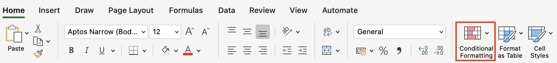
Location of Conditional Formatting in Excel’s ribbon
This feature enhances data readability, making it easier to spot trends, outliers, and key insights at a glance.
Whether you’re a beginner or an intermediate Excel user, mastering conditional formatting can significantly improve your Excel’s data analysis and decision-making processes.
In this guide, you’ll learn:
- The 5 types of conditional formatting and how to use them.
- How to create and manage conditional formatting rules.
- Best practises to avoid common pitfalls and maximise efficiency.
Let’s dive in!
The Five Types of Conditional Formatting
1. Highlight Cells Rules
Highlight Cells Rules allow you to format cells based on specific criteria, such as values greater than, less than, or equal to a certain number. This is particularly useful for identifying key data points quickly.
Examples:
- Highlight overdue dates in red.
- Color-code sales figures above a specific target in green.
How to Apply:
Select the range of cells you want to format.
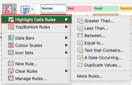
Highlighting Cell Rules
- Go to the Home tab, click Conditional Formatting, and choose Highlight Cells Rules.
- Select your desired rule (e.g., Greater Than, Less Than) and set the value.
Now that you know how to highlight specific cells, let’s move on to identifying the top and bottom values in your dataset.
2. Top/Bottom Rules
Top/Bottom Rules help you highlight the highest or lowest values, percentages, or averages in your dataset. This is ideal for performance analysis, ranking data or identifying outliers.
Examples:
- Highlight the top 10% of sales performers.
- Identify the bottom 5 lowest-scoring students in a class.
How to Apply:
- Select your data range.
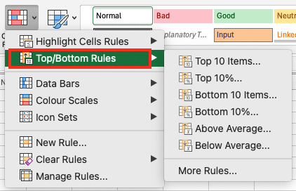
Top/Bottom Rules
- Navigate to Conditional Formatting > Top/Bottom Rules.
- Choose the rule (e.g., Top 10%, Bottom 5 Items) and customise the formatting.
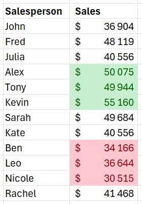
Applying the top and bottom (Source: Data Camp)
While Top/Bottom Rules are great for identifying extremes, Data Bars can help you visualise the relative size of values in your dataset.
3. Data Bars
Data Bars are visual representations of cell values, displayed as horizontal bars within the cells. They provide a quick way to compare values in a range and monitor progress.
Examples:
- Visualise inventory levels to see which items are running low.
- Track project completion percentages at a glance.
How to Apply:
- Select the cells you want to format.
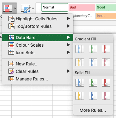
Data Bars
- Go to Conditional Formatting > Data Bars and choose a gradient or solid fill.
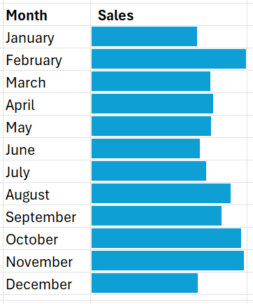
Applying Data Bars Example (Source: Data Camp)
If you want to take your data visualisation a step further, Colour Scales can help you create a heat map effect for your data.
4. Colour Scales
Colour Scales apply a gradient of colours to your data, creating a heat map effect. This is perfect for identifying trends and patterns in large datasets.
Examples:
- Apply a heat map to sales data to quickly spot high and low-performing regions.
- Use colour scales to analyse temperature variations over time.
How to Apply:
- Select your data range.
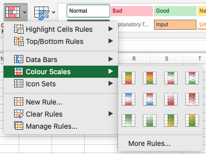
Colour Scales
- Click Conditional Formatting > Colour Scales and choose a color scheme.
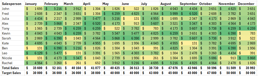
Applying Colour Scales (Source: Data Camp)
Finally, if you want to add a visual indicator to your data, Icon Sets can help you symbolise conditions like trends or priorities.
5. Icon Sets
Icon Sets use symbols like arrows, flags, or traffic lights to represent data conditions. They’re great for visualising trends or priorities.
Examples:
- Use upward and downward arrows to show sales trends.
- Add flags to indicate task priority in a project management sheet.
How to Apply:
- Select the cells you want to format.
![]()
Icon Sets
- Go to Conditional Formatting > Icon Sets and choose an icon style.
Now that you’re familiar with the 5 types of conditional formatting, let’s explore how to create and manage these rules effectively.
Creating and Managing Conditional Formatting Rules
Creating New Rules
To create custom conditional Excel formatting rules:
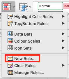
New Rule
- Select your data range.
- Go to Conditional Formatting > New Rule.
- Choose a rule type (e.g., Format only cells that contain) and set your criteria.
- Use formulas for advanced conditions, such as =AND(example of top bottom rulesA1>100, A1<200).
Managing Existing Rules
To manage rules:
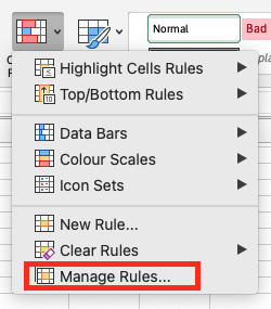
Manage Rules
- Go to Conditional Formatting > Manage Rules.
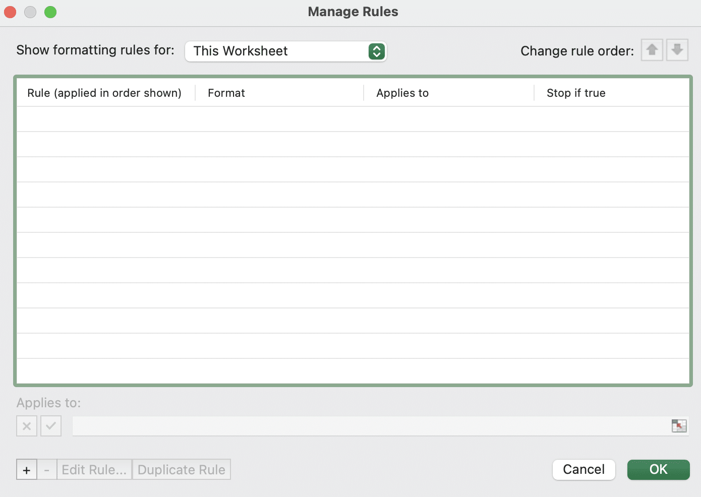
Manage Rules window
2. View, edit, or delete existing rules.
3. Adjust rule precedence by moving rules up or down in the list.
Best Practices
Here are 5 common best practices to help you avoid common pitfalls and use conditional formatting effectively:
- Avoid Over-Formatting
- Limit Rules: Apply formatting only to key data points, not entire sheets.
- Keep It Simple: Use one or two formatting styles (e.g., colors or icons) to avoid clutter.
- Test First: Try rules on a small dataset before applying them widely.
Example: Instead of applying colour scales to an entire sales report, use them only on the “Total Sales” column to highlight high and low performers.
- Use Formatting Strategically
- Highlight Key Metrics: Emphasise critical data like sales targets or deadlines.
- Identify Trends: Use color scales or data bars to show trends, like sales growth.
- Flag Exceptions: Use icons or colours to flag outliers, like low inventory.
Example: Use green for completed tasks and red for overdue ones in a project tracker. This makes it easy to see which tasks need immediate attention.
- Prioritise and Organise Rules
- Reorder Rules: Use Manage Rules to place the most important rules at the top.
- Avoid Conflicts: Ensure rules don’t overlap unnecessarily.
- Delete Unused Rules: Regularly clean up old or unnecessary rules.
Example: If you have a rule to highlight sales above 1,000 (green) and 5,000 (red), make sure the red rule is higher in the list, so it takes priority.
- Optimise for Performance
- Limit Large Datasets: Avoid formatting entire columns or rows in big datasets.
- Avoid Volatile Functions: Use TODAY() or NOW() sparingly to prevent slowdowns.
- Use Efficient Formulas: Optimise custom formulas for better performance.
Example: Instead of applying conditional formatting to an entire column of 10,000 rows, apply it only to the visible range or the most critical data points.
- Use Clear and Consistent Criteria
- Be Specific: Define exact conditions (e.g., “>100” instead of “high values”).
- Test Rules: Check rules on a small range before applying them widely.
- Document Rules: Add notes or comments to explain complex rules.
Example: Use “Format cells where the due date is earlier than today” for overdue tasks.
Now that you’ve learned how to create and manage conditional formatting rules, let’s wrap up.
Wrapping Up
Conditional formatting is a game-changer for Excel users, enabling you to transform raw data into visually appealing and actionable insights.
By mastering the 5 types of conditional formatting we’ve explored earlier, you can enhance your data visualisation in Excel and analysis skills.
Don’t be afraid to experiment with different rules and formats to see what works best for your data. With practise, you’ll be able to create dynamic, easy-to-read spreadsheets that make decision-making a breeze.
For further learning, check out these resources:
Happy formatting!
Dive Deeper into Excel
If you’re ready to learn more about Excel and its advanced techniques, @ASK Training offers a range of WSQ-accredited Microsoft Excel courses designed to help you level up your skills and productivity!
Here are a few of our popular Excel courses perfect for users of all experiences:
- WSQ Microsoft Excel Essentials: Perfect for beginners, this course covers the basics of Excel, including formatting, formulas, and data organisation.
- WSQ Microsoft Excel Intermediate: Build on your foundational knowledge with features like advanced formulas, PivotTables and more.
- WSQ Microsoft Excel Advanced: Take your expertise to the next level with advanced functions, macros, and automation techniques.
Sign up today and start transforming the way you work with data!
Related Courses
◆◆◆