
Mastering the VLOOKUP function in Excel can transform the way you handle data, making it easier to retrieve and analyse information efficiently.
Whether you’re a beginner or an intermediate user, this guide will walk you through everything you need to know. From basic syntax to advanced techniques, so you can apply VLOOKUP confidently in your work.
First, what is VLOOKUP?
Introduction to VLOOKUP
VLOOKUP (Vertical Lookup) is one of Excel’s most powerful functions, designed to search for a specific value in a table and return a corresponding result from another column.
It’s widely used for tasks like:
- Finding product prices from an inventory list.
- Matching employee IDs with their names.
- Retrieving student grades from a database.
By the end of this guide, you’ll understand how to use VLOOKUP effectively, troubleshoot common errors, and even explore advanced alternatives like XLOOKUP.
Understanding VLOOKUP Syntax and Parameters
The VLOOKUP function follows this basic structure:
=VLOOKUP(lookup_value, table_array, col_index_num, [range_lookup])
Let’s break down each parameter:
- lookup_value: The value you want to search for (e.g., a product name or ID).
- table_array: The range of cells containing the data (always include the lookup column as the first column).
- col_index_num: The column number (from the left) that contains the data you want to retrieve.
- [range_lookup]:
- FALSE for an exact match (most common).
- TRUE for an approximate match (requires the first column to be sorted).
Now the basics are clear, let’s go into the step-by-step VLOOKUP guide below.
Step-by-Step Guide to Building a VLOOKUP Formula
Follow these steps to create a VLOOKUP formula:
- Select the cell where you want the result.
- Start the formula with =VLOOKUP(.
- Enter the lookup_value (e.g., “Kiwi” or A3 for a cell reference).
- Define the table_array (e.g., A3:C10). Use absolute references ($A$3:$C$10) if copying the formula.
- Specify the col_index_num (e.g., 3 for the third column).
- Choose FALSE for an exact match or TRUE for an approximate match.
- Close the formula with ) and press Enter.
Example:
=VLOOKUP(“Kiwi”, A2:C10, 3, FALSE)
This searches for “Kiwi” in the first column of A2:C10 and returns the value from the third column.
Now, let’s take a look at some of the practical examples you can try out.
Practical Examples and Real-World Scenarios
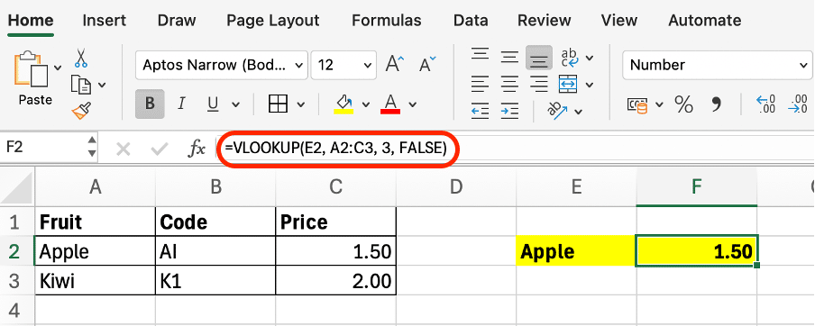
1. Basic VLOOKUP
Find the price of a fruit in a table:
| Fruit | Code | Price |
| Apple | A1 | 1.50 |
| Kiwi | K1 | 2.00 |
Formula:
=VLOOKUP("Kiwi", A2:C3, 3, FALSE)
Result: 2.00
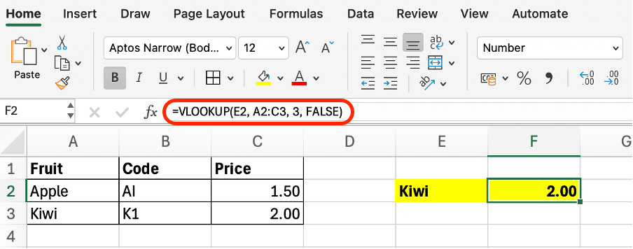
2. Dynamic Lookup with Cell References
Instead of hardcoding “Kiwi,” reference another cell (e.g., E1):
=VLOOKUP(E2, A3:C3, 3, FALSE)
Now, changing E2 updates the result automatically.
3. Partial Lookup with Wildcards
Use * to match partial text:
=VLOOKUP("App*", A2:C3, 3, FALSE)
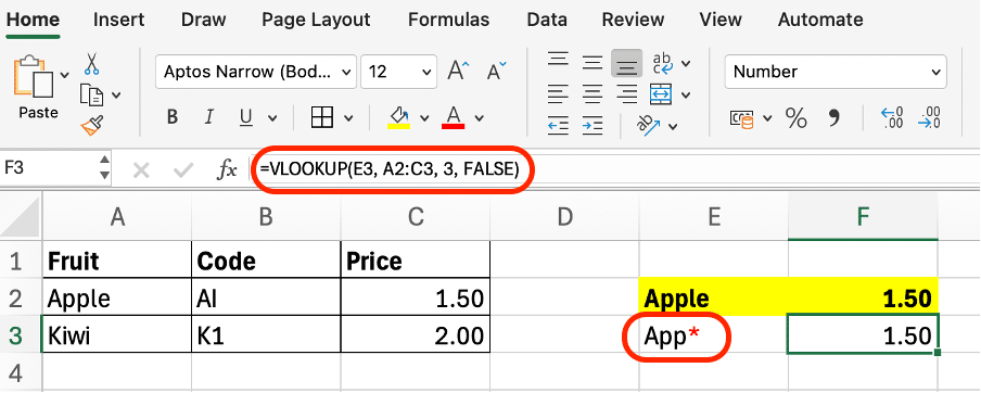
Result: 1.50 (matches “Apple”).
Troubleshooting and Error Handling
Common errors and fixes:
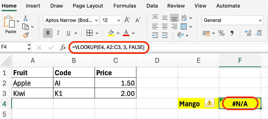
#N/A: Lookup value not found
Fix: Check for typos or use IFERROR to display a custom message:
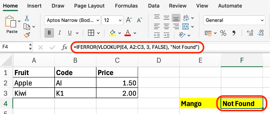
=IFERROR(VLOOKUP(E1, A2:C3, 3, FALSE), "Not Found")
#REF!: Column index exceeds table width.
- Fix: Adjust col_index_num to fit the table.
#VALUE!: Incorrect data type (e.g., searching a number in text format).
Fix: Use TRIM or VALUE to clean data.
HLOOKUP vs XLOOKUP: Alternatives to VLOOKUP
HLOOKUP
- Searches horizontally (first row instead of first column).
- Syntax:
=HLOOKUP(lookup_value, table_array, row_index_num, [range_lookup])
XLOOKUP (Modern Alternative)
- More flexible than VLOOKUP (searches in any direction, supports wildcards, and handles errors better).
- Syntax:
=XLOOKUP(lookup_value, lookup_array, return_array, [if_not_found], [match_mode], [search_mode])
Example:
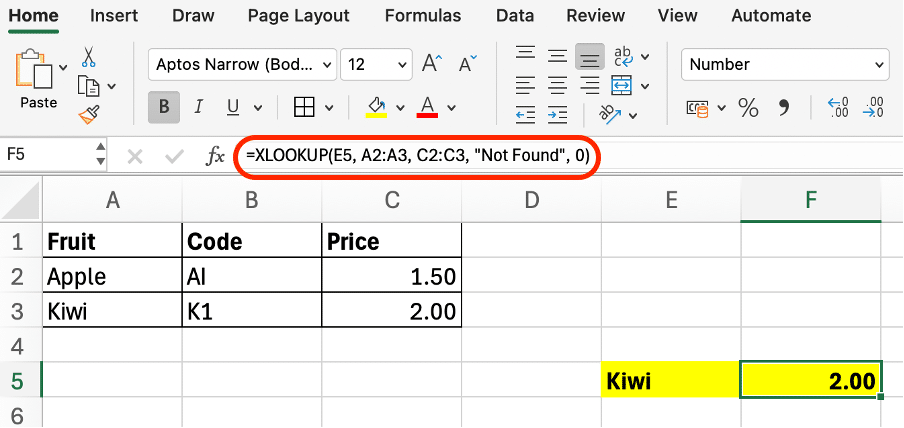
=XLOOKUP("Kiwi", A2:A3, C2:C3, "Not Found", 0)
Note: XLOOKUP is only available in Excel 365 and Excel 2021+.
Advanced Techniques
1. Two-Way Lookup with MATCH
Combine VLOOKUP + MATCH to dynamically find columns:
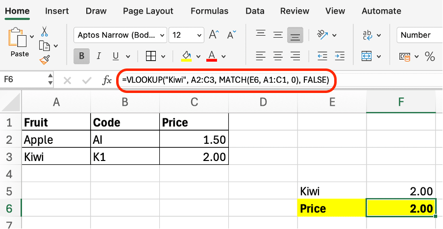
=VLOOKUP(E1, A2:C3, MATCH("Price", A1:C1, 0), FALSE)
2. Multi-Criteria Lookups
Create a helper column to concatenate criteria (e.g., =A2&B2), then use VLOOKUP on the combined key.
3. Performance Tips
- Use INDEX + MATCH for large datasets (faster than VLOOKUP).
- Avoid entire column references (e.g., A:A) to speed up calculations.
Wrapping Up
VLOOKUP is a cornerstone of Excel data analysis, enabling quick and accurate lookups. By mastering its syntax, troubleshooting errors, and exploring advanced techniques, you’ll streamline your workflows and handle data like a pro.
Ready to practise? Open Excel and try these examples in your own workbook! For further learning, check out these helpful resources:
- Microsoft Support (VLOOKUP function)
- Ablebit’s Excel VLOOKUP tutorial for beginners
- Kevin Stratvert’s VLOOKUP Youtube tutorial
Have fun practising!
Want to Be Excellent in Excel?
@ASK Training also offers a variety of Microsoft Excel courses! Whether you’re a beginner or an advanced user, our expert-led training will help you master functions like VLOOKUP, pivot tables, macros, and more.
Here are a few popular ones for you:
- WSQ Microsoft Excel Essentials: Learn the basics of Excel, from formulas to formatting, for efficient spreadsheet use.
- WSQ Microsoft Excel Intermediate: Build on your skills with advanced functions and data analysis tools.
- WSQ Microsoft Excel Advanced: Master advanced features like macros and pivot tables for automation and in-depth data analysis.
- Microsoft Excel Advanced Formulas & Functions: Perform advanced searching and data retrieval with Lookup functions.
Explore more of our Excel courses today and unlock the full potential of your data skills!
Related Courses
- WSQ Microsoft Excel Essentials
- WSQ Microsoft Excel Intermediate
- WSQ Microsoft Excel Advanced
- Microsoft Excel: Advanced Formulas and Functions
◆◆◆