
Have you ever spent way too much time scrolling through endless Excel rows trying to find a specific piece of data? Or worse—used VLOOKUP only to realise it can’t search to the left of your lookup column?
You’re not alone. Many Excel users hit these frustrations daily, but there’s a better way: INDEX and MATCH.
Think of INDEX and MATCH as Excel’s dynamic duo for finding data. While VLOOKUP is like a one-way street (only searching right), INDEX MATCH in Excel gives you the freedom to search in any direction—left, right, up, down—and even handle multiple criteria with ease.
Whether you’re tracking sales, managing inventory, or analysing student grades, mastering these functions will save you time and headaches.
In this guide, we’ll break down the Excel INDEX function and Excel MATCH function in simple terms, show you how to combine them like a pro, and walk you through real-world examples. So, you can stop wasting time on manual searches and start working smarter!
Let’s dive in.
Understanding INDEX and MATCH Functions
The INDEX Function
The INDEX function retrieves a value from a specified position within a range. Its syntax is:
=INDEX(array, row_num, [column_num])
- array: The range of cells containing the data.
- row_num: The row number from which to fetch the value.
- [column_num]: (Optional) The column number if the range is multi-dimensional.
Example:
=INDEX(A2:B10, 3, 2)
This returns the value in the 3rd row and 2nd column of the range A2:B10.
The MATCH Function
The MATCH function searches for a value and returns its relative position in a range. Its syntax is:
=MATCH(lookup_value, lookup_array, [match_type])
- lookup_value: The value you want to find.
- lookup_array: The range where Excel should search.
- [match_type]:
- 0 for an exact match (most common).
- 1 for approximate match (values sorted in ascending order).
- -1 for approximate match (values sorted in descending order).
Example:
=MATCH("Apple", A2:A10, 0)
This returns the position of “Apple” in the range A2:A10.
Now that you understand each function individually, let’s explore how combining them unlocks Excel’s full lookup potential.
Combining INDEX and MATCH for Lookups
The real power of INDEX MATCH in Excel comes from merging these two functions. The combined formula looks like this:
=INDEX(return_range, MATCH(lookup_value, lookup_range, 0))
Here’s how it works:
- MATCH finds the position of the lookup value.
- INDEX uses that position to retrieve the corresponding value from another column.
Example:
Suppose you have a list of products (A2:A10) and their prices (B2:B10). To find the price of “Laptop,” use:
=INDEX(B2:B10, MATCH("Laptop", A2:A10, 0))
Why is this better than VLOOKUP?
- Works left-to-right and right-to-left.
- Handles dynamic ranges efficiently.
- More reliable with large datasets.
Ready to build your own formula? Follow these steps.
Step-by-Step Instructions to Build an INDEX/MATCH Formula
Here’s a step-by-step guide on how to use INDEX and MATCH:
- Identify the Lookup Value: Determine what you’re searching for (e.g., a product name).
- Define the Lookup Range: Select the column where the lookup value exists.
- Define the Return Range: Choose the column containing the data you want to retrieve.
- Insert MATCH: Use MATCH to find the position of the lookup value.
- Insert INDEX: Use INDEX to pull the corresponding value from the return range.
- Test the Formula: Verify results and adjust ranges if needed.
Example:
=INDEX(C2:C100, MATCH("Project X", A2:A100, 0))
Let’s apply this to real-world scenarios.
Practical Examples and Real-World Scenarios
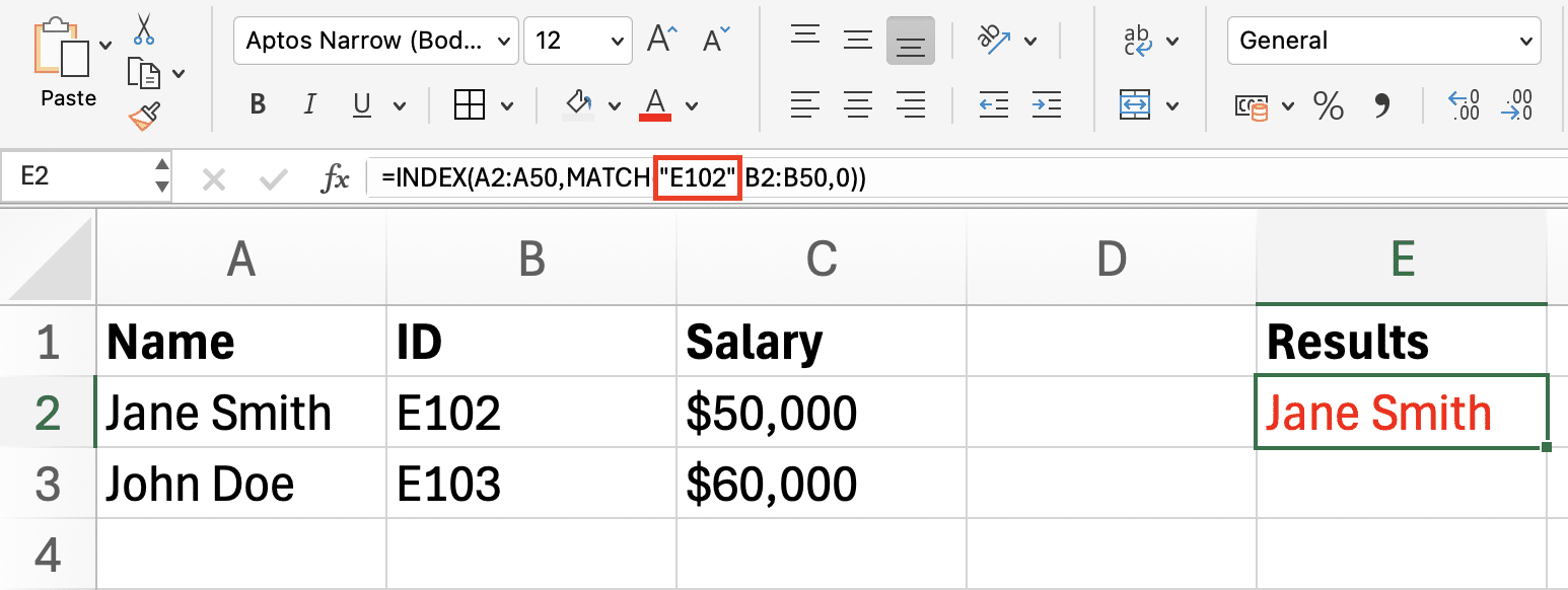
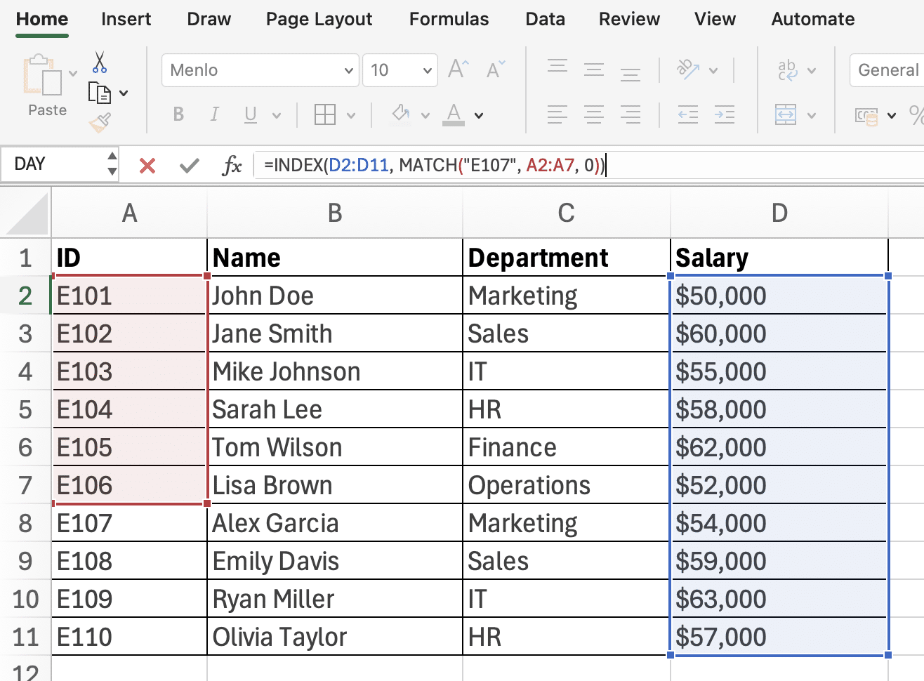
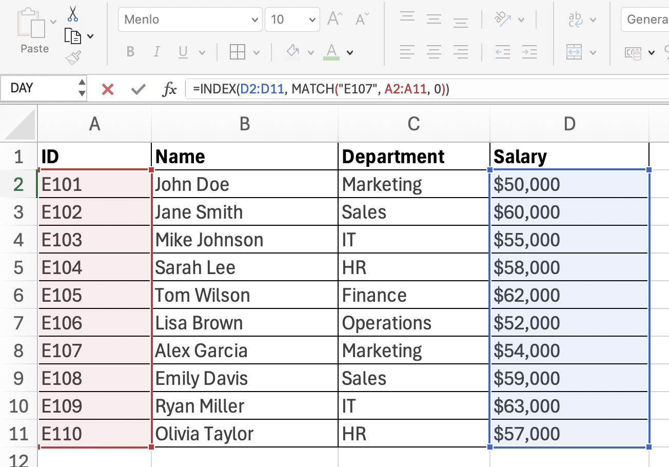
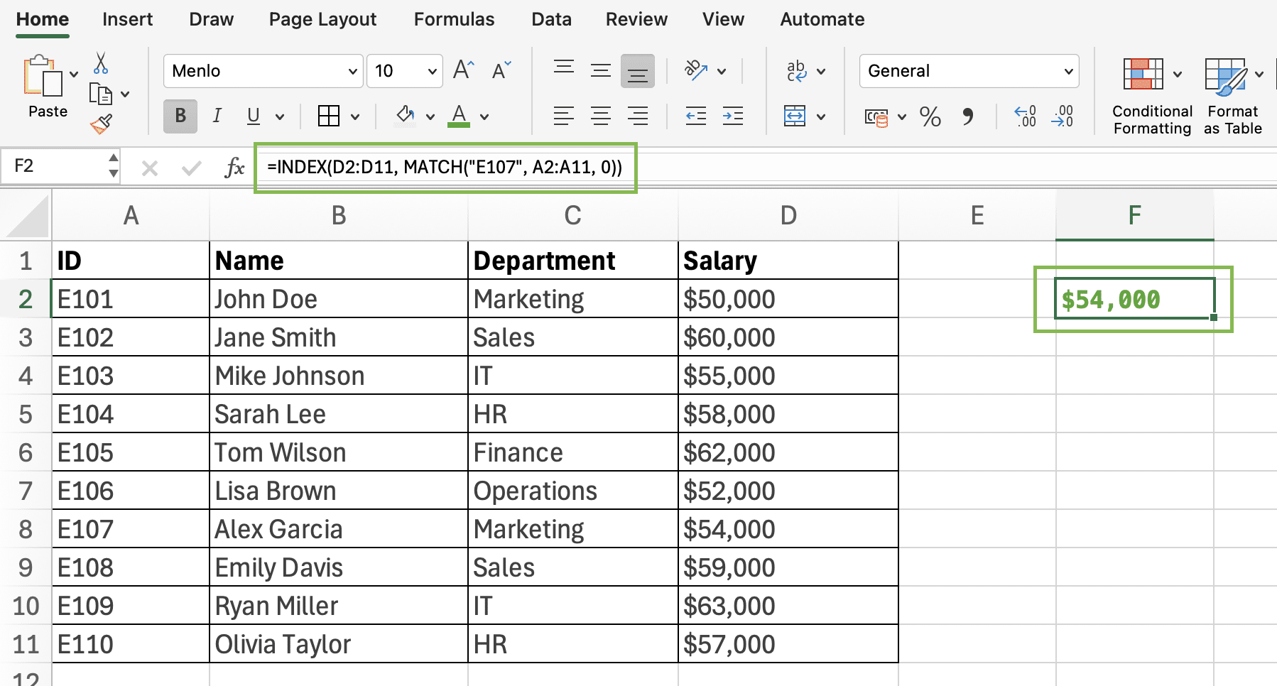
1. Basic Lookup
Find an employee’s salary based on their ID:
=INDEX(D2:D50, MATCH("E102", A2:A50, 0))

2. Dynamic Lookup
Use a cell reference for flexibility:
=INDEX(D2:D50, MATCH(H1, A2:A50, 0))

(Where D2 to D50 may contain the lookup value, and in this case, the found value is in D2.)
3. Multi-Criteria Lookup
Combine criteria with helper columns or concatenation:
=INDEX(C2:C100, MATCH(1, (A2:A100="North")*(B2:B100="Q1"), 0))
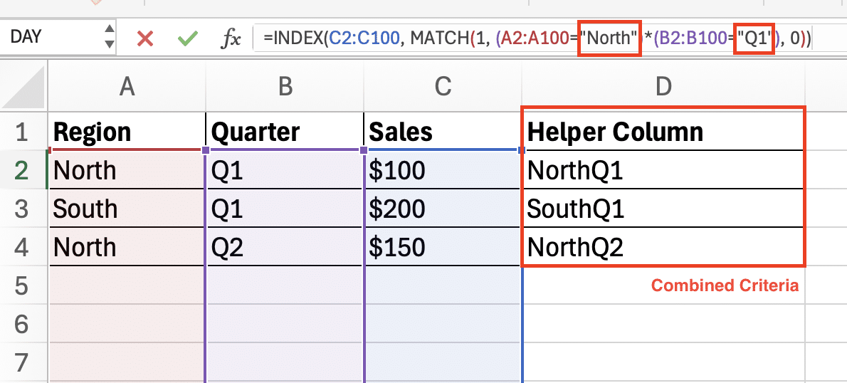
Enter as an array formula with Ctrl+Shift+Enter in older Excel versions, Excel 365 handles this automatically.
4. Reverse Lookup
Retrieve a name from an ID (where IDs are to the right of names):
=INDEX(A2:A50, MATCH("ID102", B2:B50, 0))
What if your formula returns an error? Knowing how to avoid INDEX MATCH errors can help you spot missing lookup values, mismatched ranges, and formula issues before they affect your results.
Troubleshooting and Error Handling
1. #N/A Error: The lookup value isn’t found.
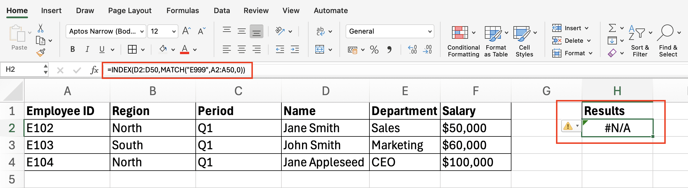
Before
Fix: Verify spelling or use IFERROR for a cleaner output:
=IFERROR(INDEX(B2:B10, MATCH("Value", A2:A10, 0)), "Not Found")

After
2. Incorrect Results: Faulty formula from mismatched ranges.

Mismatch Formula
Fix: Ranges must match in size!
After Fixing
Now that we’ve gone through examples of troubleshooting errors, how does INDEX/MATCH compare to other Excel lookup functions?
INDEX/MATCH vs VLOOKUP: Which Should You Use?
| Feature | INDEX/MATCH | VLOOKUP | XLOOKUP |
| Lookup Direction | Left, right, or vertical | Right-only | Any direction |
| Insert/Delete Columns | Unaffected | Breaks if columns are added/deleted | Unaffected |
| Approximate Match | Supported (match_type 1/-1) | Supported | More intuitive syntax |
| Multiple Criteria | Yes (with array formulas) | No | Yes (native support) |
| Error Handling | Manual (IFERROR needed) | Manual | Built-in (e.g., “Not Found” message) |
| Speed | Fast with defined ranges | Slows with big data | Optimised for performance |
When to Use Each:
INDEX/MATCH is best for:
- Legacy Excel versions (pre-2019)
- Complex lookups (left searches, 2-way lookups)
- Large datasets where you need control over ranges
VLOOKUP is best for:
- Quick, simple right-only lookups
- Beginners learning basic lookup concepts
- Legacy workbooks where compatibility is critical
XLOOKUP is best for:
- Excel 365/2021 users
- Simplified syntax and built-in error handling
- Dynamic array formulas
Key Takeaway: INDEX/MATCH remains the most flexible option for all Excel versions, but XLOOKUP is the future if you have access to it.
Advanced Techniques & Tips for Effective Use
While the basic combination is powerful, these advanced techniques will help you solve more complex problems. Let’s see how they work:
1. Two-Way Lookups (Row & Column Search)
Need to find a value at the intersection of a specific row and column? Combine INDEX with two MATCH functions:
=INDEX(data_range, MATCH(row_value, row_header_range, 0), MATCH(column_value, column_header_range, 0))
Example:
Find the sales amount for “Product A” in “Q2”:
=INDEX(B2:E10, MATCH("Product A", A2:A10, 0), MATCH("Q2", B1:E1, 0))
Why it’s better than VLOOKUP?
- Works both horizontally and vertically.
- Doesn’t break if columns are rearranged.
2. Multi-Criteria Lookups
When one condition isn’t enough, use these methods:
Option 1: Helper Column
- Add a new column combining your criteria (e.g., =A2&B2).
- Use INDEX/MATCH on this column:
=INDEX(C2:C100, MATCH("Criteria1Criteria2", helper_column, 0))
Option 2: Array Formula (Legacy Excel)
=INDEX(C2:C100, MATCH(1, (A2:A100="North")*(B2:B100="Q1"), 0))
(Press Ctrl+Shift+Enter in older Excel versions.)
Option 3: XLOOKUP (Excel 365)
Simpler with native multi-criteria support:
=XLOOKUP("North"&"Q1", A2:A100&B2:B100, C2:C100)
3. Performance Tips for Large Datasets
- Avoid entire columns: Use A2:A1000 instead of A:A.
- Use Tables: Structured references (e.g., Table1[Sales]) auto-adjust and improve readability.
- Limit array formulas: They slow down calculations in big files.
- Sort data for approximate matches: If using match_type 1/-1, sort your lookup column first.
Before we wrap this article up, here are a few INDEX MATCH tutorials you can explore:
- Corporate Finance Institute INDEX MATCH tutorial
- Ablebits on how INDEX MATCH works
- Microsoft Support on INDEX MATCH
Wrapping Up
Mastering INDEX and MATCH unlocks Excel’s full potential for flexible, powerful lookups. Here’s what you’ve learned:
- Basics: How each function works individually and combined.
- Real-world uses: From simple lookups to multi-criteria searches.
- Troubleshooting: Fixing #N/A errors and optimising performance.
- Advanced tricks: Two-way lookups and dynamic ranges.
Your Next Steps:
- Practice with your own data, try replacing VLOOKUPs with INDEX/MATCH.
- Experiment with two-way lookups for reports/dashboards.
- Explore further: Learn about XLOOKUP (if you have Excel 365) or dynamic arrays.
Remember: INDEX/MATCH is a skill you’ll use for years, whether analysing budgets, managing inventory, or creating complex models.
Start small, and soon you’ll wonder how you ever used Excel without it!
Ready to Excel Like a Pro?
Now that you’ve unlocked the power of INDEX & MATCH, go further with @ASK Training’s range of Microsoft Excel courses suitable for beginners and pro users!
Some of our popular Excel courses include:
- WSQ Microsoft Excel Essentials: Master the fundamentals, from formulas to formatting in this hands-on beginner course.
- WSQ Microsoft Excel Intermediate: Master data management, advanced formulas (VLOOKUP/IF), error tracing, and dynamic reporting.
- Microsoft Excel Advanced: Level up with PivotTables, data analysis, and dynamic functions for workplace efficiency.
- Microsoft Excel: Advanced Formulas and Functions: Transform raw data into insights with advanced Lookup, Statistical, and Text functions
Enrol with us today! Don’t just learn Excel, master it!
Related Courses
- WSQ Microsoft Excel Essentials
- WSQ Microsoft Excel Intermediate
- Microsoft Excel Advanced
- Microsoft Excel: Advanced Formulas and Functions
◆◆◆