Step-by-Step Guide to Creating Data Models in Power Pivot

In today’s world of data analysis, being able to work quickly and accurately is essential. This is where Power Pivot, a feature in Microsoft Excel, comes in to help.

Power Pivot lets you handle large amounts of data, connect tables together, and perform advanced calculations – all without needing to be a data expert.

For example:

A business analyst can use Power Pivot to combine sales data from different regions and create one comprehensive report.
A student can use it to compare multiple datasets for a school project.

These examples show how Power Pivot simplifies Excel data analysis, saving time, reducing errors, and making working with data much easier for everyone. It’s a powerful tool for both professionals and beginners looking to learn more advanced Excel features.

In this guide, we’ll show you step-by-step how to create data models in Power Pivot, manage, and optimise them so you can start analysing your data like a pro.

Let’s dive in! To begin, let’s understand the key building blocks of Power Pivot: Data Models.

1. Understanding Data Models in Power Pivot

A data model is like a blueprint that organises your data so Excel can understand it better. Power Pivot uses data models to connect tables, making it easy to perform advanced analysis without having to manually link data yourself.

Key Parts of an Excel Data Model

Tables: Think of these as Excel sheets that hold your raw data, like sales numbers or customer details.
Relationships: These are the connections between tables, like linking a “Customer ID” in one table to a “Customer ID” in another.
Fields: These are the columns in your tables, such as “Date,” “Product Name,” or “Sales Amount,” which you’ll use in your analysis.

In regular Excel, your data often stays in separate sheets, making it hard to work with. Power Pivot brings all the data together in one model, saving you time and effort.

Why Relationships Matter

By connecting tables through relationships, Power Pivot allows you to analyse data across multiple sources without repeating or duplicating information. For example, you can link sales data to a product catalogue and instantly see which products are performing best.

Now that you understand what data modelling in Excel is and why it’s important, let’s learn how to prepare your data to ensure everything works smoothly in Power Pivot.

2. Preparing Your Data

Before you can start building a data model in Power Pivot, you need to make sure your data is clean and organised. Here’s how to prepare your data step by step:

Steps for Preparation

Remove duplicates: Check for and eliminate duplicate rows to ensure your data is accurate.
Standardise formats: Make sure dates, numbers, and text are consistent throughout your dataset (e.g., use the same date format everywhere)
Create unique identifiers: Use primary keys (e.g., order ID, employee ID) to link data between tables. These act like a glue that holds your relationships together.

Helpful Tools in Excel

Remove Duplicates: Use this feature under the Data tab to clean up repeated entries.
Text to Columns: Break apart data in a single column into multiple columns (e.g., splitting full names into first and last names).
Flash Fill: Quickly fill in patterns, like formatting phone numbers or extracting text.

By cleaning your data first, you’ll make sure everything runs smoothly when you start creating your data model. Taking the time to do this upfront saves a lot of headaches later!

With your data now clean and organised, the next step is to enable Power Pivot in Excel and start building your data model.

3. Enable Power Pivot

Power Pivot might not be turned on in Excel by default, and it’s important to note that Power Pivot is not available for Mac users. If you’re using Windows, follow these simple steps to enable Power Pivot:

How to Check and Enable Power Pivot

You can also refer to this Microsoft guide for detailed instructions.

1. Check for Power Pivot

Look at your ribbon (the menu at the top of Excel). If you see a tab called Power Pivot, it’s already enabled.

2. Enable Power Pivot (if it’s missing):

For Office 365/Excel 2019: Go to File > Options > Add-Ins. Select COM Add-ins from the dropdown and check “Microsoft Power Pivot for Excel.”
For older versions: Follow the version-specific instructions provided in the Microsoft guide linked above.

Here’s what it looks like to navigate to Options and enable the Add-In:

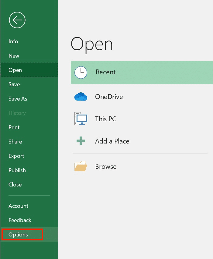
Go to File and Click ‘Options’ at the bottom (Desktop Version)

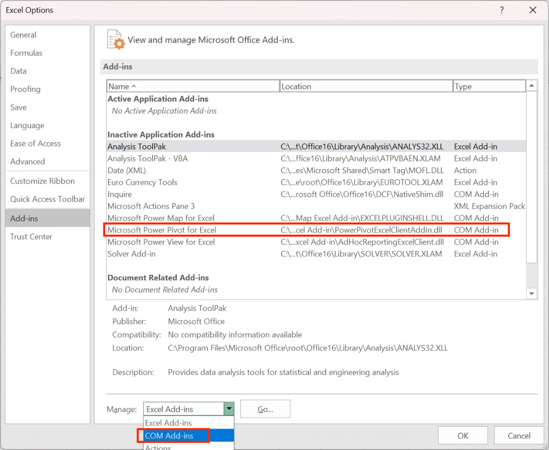
Select COM Add-Ins (Desktop Version)

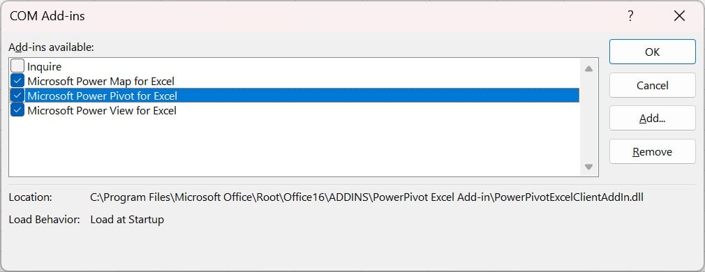
Check Microsoft Power Pivot for Excel (Desktop Version)

3. Access the tab: Once enabled, you’ll see the Power Pivot tab in your ribbon at the top of Excel.

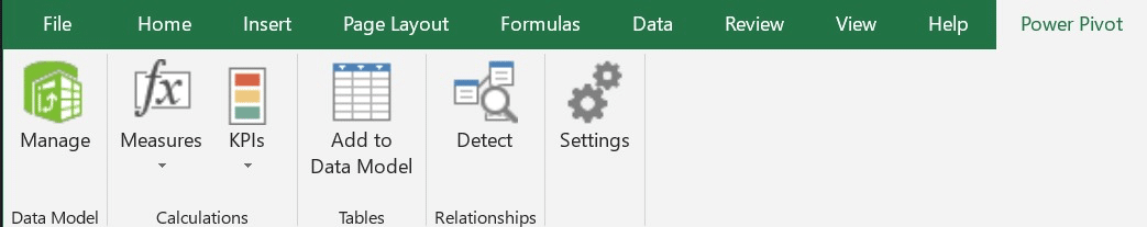
Power Pivot Tab

Important Note for Mac Users

Power Pivot is a Windows-only feature, so Mac users will need to explore alternative solutions like Power BI or other third-party tools.

Now that Power Pivot is enabled, let’s move on to importing your data and getting it ready for analysis.

4. Importing Data in Power Pivot

Power Pivot allows you to bring in data from different sources and combine them into one model. This makes it easy to analyse multiple datasets in one place. Here’s how you can import data:

Excel tables: Use structured tables for a seamless import.
Databases: Connect directly to SQL or Access databases.
CSV files: Import datasets saved in CSV format.

Steps to Import Data

1. Power Pivot by clicking on the Power Pivot tab in your Excel ribbon.

2. Select Manage to open the Power Pivot window.

3. Click on Get External Data and choose the sources you want to import data from (e.g., Excel tables, databases, or CSV files).

Here’s what it looks like in Excel:

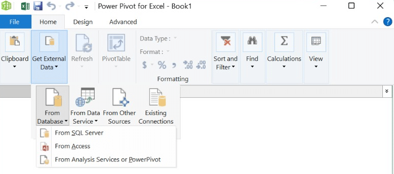
Import Data (Desktop Version)

4. When prompted, make sure to select the option to Add data to the Data Model for seamless integration into Power Pivot.

Tip: You can practise importing data using sample property sales data from the NSW Residential Property Trends Model. This dataset includes prices, locations, and property types that are already structured into tables, making it easy to work with in Power Pivot.

With your data successfully imported, the next step is to create relationships between tables to connect your data and unlock deeper analysis.

5. Creating Relationships

Once your data is imported, you’ll need to create relationships between your tables. Relationships allow Power Pivot to link data across tables ensuring accurate analysis.

Why Relationship Matter:

If relationships are missing or mismatched, Power Pivot might produce incorrect calculations or incomplete data. For example, without linking a “Region ID” in one table to the same field in another, Power Pivot won’t know how to connect the data.

Steps to Create Relationships

Open the Power Pivot window.
Click on Diagram View to see your tables visually.
Drag and drop common fields (e.g., “Region ID” or “Order ID”) from one table to the matching field in another.
Validate the relationships by ensuring they reflect a one-to-many.

Here’s what Diagram View looks like:

Diagram View (Desktop Version)

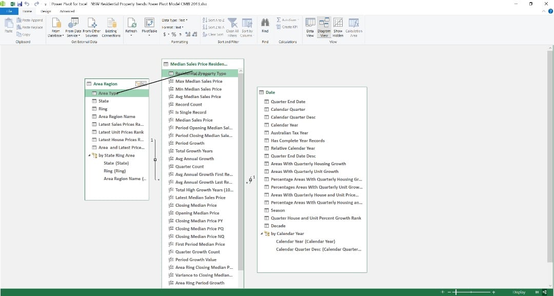
Drag & Drop Example (Desktop Version)

Tip:

If your relationships are mismatched, Power Pivot might show errors or incomplete PivotTables.
Always double-check that the linked fields share the same format (e.g., both as numbers or text).

By creating proper relationships, you can ensure your data in integrated correctly, allowing for advanced and reliable analyses.

Now that your tables are linked through relationships, you can start building calculated columns and measures to gain valuable insights from your data.

6. Building Calculated Columns and Measures

Power Pivot uses DAX (Data Analysis Expressions) to perform custom calculations on your data. If you’re new to DAX, don’t worry! It’s beginner-friendly. You can start with simple functions like SUM, AVERAGE, or IF to gain confidence.

What Are Calculated Columns and Measures?

Calculated Columns: These are new columns added to your table that perform a calculation for each row.
Measures: These are formulas used to calculate one overall result, like totals or averages, for your entire dataset.

Examples

Calculated Column

Imagine you have a table of property sales, and you want to calculate the “Price per Square Meter.” You can create a calculated column by dividing the total price by the area of each property using the formula:

Price per Square Meter = Sales[Total Price] / Sales[Area]

Measure

If you want to find the total sales revenue for all properties, use a measure. This calculates one result for the entire table.

Formula:

Total Revenue = SUM(Sales[Total Price])

When Should You Use Each?

Calculated Columns

Use when you need to calculate values row by row.
Example: Price per square meter for individual properties.

Measures

Use for aggregated results like totals or averages.
Example: Total revenue or average price across all properties.

Here’s an example of a calculated column in the NSW Residential Property Model:

This column ranks house prices by area using a DAX formula

(Source: CMBI)

For more advanced learning, explore resources like Microsoft’s official DAX documentation or beginner-friendly tutorials available online.

Now that you’ve learned how to enhance your data with calculated columns and measures, let’s bring your data model to life with PivotTables for dynamic analysis.

7. Using Data Model in PivotTables

Once your data model is ready, you can use it in PivotTables to quickly analyse your data and create useful reports. PivotTables lets you turn your data into summaries, charts, and insights with just a few clicks.

Steps To Try

1. Insert a PivotTable:

Go to the ribbon and click on Insert > PivotTable.
Select Use this workbook’s Data Model as the data source.

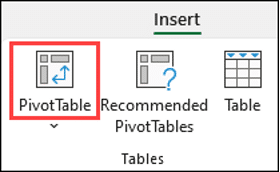
PivotTable in Insert Ribbon

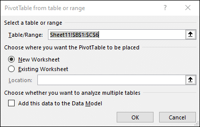
Get from Data Model Window

2. Drag and Drop Fields:

In the PivotTable Field List, drag fields (columns) into the Rows, Columns, Values, and Filters
For example, drag “Region” to Rows and “Sales Amount” to Values to see total sales by region.

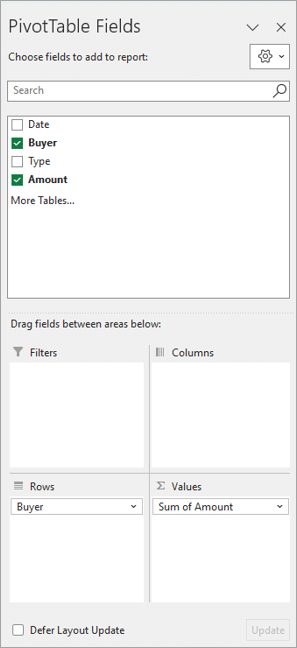
Field List Window Example

(Source: Microsoft)

3. Analyse Your Data:

Create reports like “Total Sales by Region” or “Yearly Growth.”
Add slicers or filters to make your reports interactive and easy to explore.

Tip: Practice dragging and dropping different fields to see how the Pivot Table changes. It’s an easy way to learn!

Now that your data model is set up and enhanced with calculated columns and measures, it’s time to turn your data into actionable insights using PivotTables.

8. Optimising Your Data Model

When working with large datasets, keeping your data model efficient ensures it runs smoothly and doesn’t slow down Excel.

Simple Tips to Optimise:

Remove Unnecessary Data:

Only keep the columns and tables you need. For example, if you’re not analysing “Phone Numbers,” don’t import that column.

Use Clear Names:

Rename your tables and fields to something easy to understand, like changing “Tbl_1” to “Sales Data.”

Organise with Diagram View:

Open Diagram View in Power Pivot to see all your tables and relationships visually. Arrange them neatly and check for errors.

Why Optimise?

Optimised models are faster, use less memory, and are easier to work with—especially for beginners.

As your data models grow, optimising them becomes essential to ensure they remain efficient, organised, and easy to work with.

9. Common Issues and Solutions

Power Pivot is powerful, but it can come with challenges. Here are common issues and how to fix them:

Data Refresh Errors:

Issue: Data doesn’t update when you refresh the model.
Fix: Make sure the original data source (e.g., your Excel file or database) is still available and hasn’t moved.

Relationship Problems:

Issue: Your tables don’t connect properly, and the data looks wrong.
Fix: Check that linked fields have the same format (e.g., both as text or both as numbers).

Save Frequently:

Issue: Losing work due to crashes or mistakes.
Fix: Save your progress often while working on your model.

Tip: Don’t panic! Most errors are small and easy to fix once you understand where the problem lies.

Even with the best preparation and optimization, occasional challenges may arise when working with Power Pivot. Here’s how to troubleshoot common issues.

10. Advanced Techniques

Once you’re comfortable with the basics, you can explore advanced features to make your models even more powerful.

Ideas to Try

Learn Advanced DAX Formulas:

Use formulas like CALCULATE (to customise filters) or FILTER (to narrow down data).
Example: Calculate the total sales for a specific region using CALCULATE(SUM(Sales[Total Sales]), Sales[Region] = “North”).

Combine Data from Multiple Sources:

Link Excel tables, databases, or CSV files into one model to analyse everything in one place.

Explore More Tools:

If you enjoy Power Pivot, try Power BI! It’s a free Microsoft tool for even more advanced data analysis and visualisation.

Tip for Beginners: Focus on mastering the basics first. Advanced features will make more sense once you’re confident with the fundamentals

Wrapping Up

Power Pivot transforms how Excel users approach data analysis by allowing them to handle massive datasets, create relationships between tables, and perform advanced calculations that go beyond traditional Excel capabilities.

By following this guide, you can create robust data models, establish meaningful relationships, and derive powerful insights.

Start practising with your datasets today to build confidence and master this game-changing Excel feature. Check out helpful Power Pivot tutorials online to assist with your practises!

Interested in Learning More?

While this guide provides a solid foundation, real-world application is key! Explore @ASK Training’s Microsoft Excel courses on Power Pivot that cover fundamental concepts to advanced techniques like Time Intelligence DAX!

Perfect for beginners and advanced users, our courses include:

Get in touch with us today to empower your data analysis skills and stay ahead of the curve!

Related Courses

◆◆◆